What Does It Mean to Seasonally Adjust Data
Seasonally-Adapted Data: What it Actually Means
Thursday, March 31, 2022
This paper provides a brief overview of what it means when information are seasonally-adapted and describes the advantages of using seasonally adjusted information to examine changes in data. The Bureau of Transportation Statistics' airline data are used as an illustrative example. For the most contempo information and model used for seasonal aligning, visit: https://data.bts.gov/Research-and-Statistics/Transportation-Services-Index-and-Seasonally-Adjus/bw6n-ddqk
Statisticians employ the process of seasonal-adjustment to uncover trends in data. Monthly information, for instance, are influenced by the number of days and the number of weekends in a calendar month as well equally by the timing of holidays and seasonal activity. These influences make it difficult to see underlying changes in the data. Statisticians utilize seasonal adjustment to control for these influences.
Controlling of seasonal influences allows measurement of real monthly changes; brusque and long term patterns of growth or decline; and turning points. Information for one month can be compared to data for any other month in the series and the data series can be ranked to find high and depression points. Whatsoever observed differences are "real" differences; that is, they are differences brought almost by changes in the data and not brought about past a change in the number of days or weekends in the month, the occurrence or non-occurrence of a holiday, or seasonal activity.
Seasonal adjustment is used for many time-series such information sets equally the Agency of Economical Assay' quarterly Gross Domestic Production (Gross domestic product), the Census Bureau's U.S. International Trade in Goods and Services, New Residential Sales and New Residential Construction, and the Agency of Labor Statistics' monthly Employment State of affairs Summary.
Transportation data tend to be highly seasonal. Revenue passenger-miles (RPMs), a measure out of air travel demand, are strongly afflicted by seasonal activity. RPMs tend be to college in summer months because of vacation-related travel and tend to rise in the month containing Easter, which changes twelvemonth-to-yr. These are normal, intra-yearly (seasonal) changes, which tin exist modeled so equally to uncover underlying changes in the information itself – for case, changes in RPMs after nine/11.
RPMs viewed over a xiv-twelvemonth menstruum illustrate the differences betwixt unadjusted and seasonally-adapted data. Betwixt January 2000 and January 2014, unadjusted RPMs were the highest in July 2013, followed by three other Julys. After seasonal aligning, those Julys rank significantly lower, every bit the seasonal adjustment process controls for seasonal motion in travel. The seasonally-adapted information bear witness that all of the superlative 5 months between January 2000 and January 2014 took identify in the months of Nov through January and the peak calendar month was January 2014, followed by the months of December and November 2013. (See Table 1)
TABLE 1. MONTHS WITH THE HIGHEST Acquirement Passenger MILES (RPMS) (TOP 10)
(Jan. 2000 – January. 2014)
Ranked past Unadjusted RPMs (thousands)
| Rank (unadjusted) | Date | Unadjusted | Adjusted | Rank (adjusted) |
|---|---|---|---|---|
| 1 | July-2013 | 81,267,865 | 69,898,894 | 12 |
| 2 | July-2011 | fourscore,361,588 | 68,641,404 | 35 |
| three | July-2007 | 79,865,224 | 69,112,655 | 26 |
| v | August-2013 | 79,331,300 | 70,281,149 | half dozen |
| 6 | July-2008 | 78,772,769 | 67,668,170 | 55 |
| 7 | August-2007 | 78,314,560 | 69,796,323 | xv |
| 8 | July-2010 | 78,192,819 | 66,472,200 | 71 |
| 9 | June-2013 | 77,864,371 | 70,231,530 | seven |
| ten | August-2012 | 77,738,861 | 68,705,504 | 33 |
Ranked by Seasonally-adjusted RPMs (thousands)
| Rank (adjusted) | Appointment | Adapted | Unadjusted | Rank (unadjusted) |
|---|---|---|---|---|
| 1 | January-2014 | 70,953,068 | 64,071,382 | 79 |
| 2 | December-2013 | 70,894,235 | 70,372,049 | 38 |
| iii | November-2013 | 70,812,961 | 63,029,023 | 90 |
| five | November-2007 | seventy,340,924 | 65,333,114 | 67 |
| 6 | Baronial-2013 | 70,281,149 | 79,331,300 | 5 |
| 7 | June-2013 | seventy,231,530 | 77,864,371 | 9 |
| viii | May-2013 | lxx,067,688 | 72,980,842 | 26 |
| ix | September-2013 | 70,065,441 | 66,575,134 | 62 |
| 10 | February-2008 | 70,043,143 | 60,578,996 | 111 |
NOTES:Revenue rider miles from all U.South. air carrier domestic and international, scheduled passenger flights
SOURCE: U.South. Department of Transportation, Bureau of Transportation Statistics, https://world wide web.transtats.bts.gov/OSEA/TSI/ equally of May 9, 2014
Available seat-miles (ASMs), a measure out of airline chapters, also illustrate the differences between unadjusted and seasonally-adjusted information. ASMs are highly seasonal and as a result, it is hard to discern trends in ASMs without seasonal adjustment. The seasonally-adjusted numbers bear witness that no month since May 2008 has broken into the tiptop 10 months for capacity. Airlines reduced capacity in 2008 in response to the recession and to the increase in the toll of fuel; airlines accept non all the same returned to capacity levels operated earlier these events. Unadjusted numbers suggest otherwise; they show that airlines operated at highest capacity in July 2013. That month, nonetheless, ranks lower after seasonal adjustment, considering of the control for the natural increase of airline rider travel in July. (See Tabular array 2)
TABLE two. MONTHS WITH THE HIGHEST AVAILABLE SEAT MILES (ASMS) (Top x)
(Jan. 2000 – January. 2014)
Ranked past Unadjusted ASMs (thousands)
| Rank (unadjusted) | Date | Unadjusted | Adjusted | Rank (adapted) |
|---|---|---|---|---|
| 1 | July-2013 | 93,812,376 | 84,551,333 | 28 |
| 2 | July-2008 | 93,730,360 | 85,809,078 | 15 |
| iii | July-2007 | 92,900,560 | 85,672,566 | 17 |
| 5 | July-2011 | 92,505,512 | 83,345,640 | 52 |
| half dozen | August-2013 | 92,159,056 | 84,870,242 | 24 |
| vii | July-2012 | 91,937,384 | 82,707,051 | 76 |
| 8 | August-2008 | 91,768,768 | 84,943,658 | 21 |
| 9 | July-2005 | 90,483,560 | 84,390,298 | 33 |
| 10 | July-2006 | ninety,151,120 | 83,563,082 | 48 |
Ranked by Seasonally-adjusted ASMs (thousands)
| Rank (adjusted) | Date | Adjusted | Unadjusted | Rank (unadjusted) |
|---|---|---|---|---|
| 1 | November-2007 | 88,323,472 | 83,926,904 | 56 |
| 2 | December-2007 | 88,107,858 | 87,368,016 | 28 |
| 3 | January-2008 | 88,006,180 | 85,823,992 | 38 |
| 5 | October-2007 | 87,709,527 | 86,936,672 | 31 |
| six | March-2008 | 87,484,395 | 89,259,056 | 17 |
| 7 | September-2007 | 87,059,611 | 84,375,736 | 52 |
| 8 | May-2008 | 86,784,781 | 88,697,896 | twenty |
| 9 | Apr-2008 | 86,626,984 | 85,702,944 | 40 |
| 10 | Jan-2007 | 86,355,182 | 84,354,432 | 53 |
NOTES: Available seat miles from all U.South. air carrier domestic and international, scheduled passenger flights
SOURCE: U.S. Department of Transportation, Bureau of Transportation Statistics, https://world wide web.transtats.bts.gov/OSEA/TSI/asonalized_data as of May 9, 2014
SEASONAL ADJUSTMENT IN TRANSPORTATION
Seasonal aligning is the process of estimating and removing move in a time-serial acquired by regular seasonal variation in action, e.yard., an increase in air travel during summer months. Agenda furnishings (trading days and holidays) often innovate additional movement in the time-series, and information outliers may disrupt movement altogether. Both calendar effects and data outliers make it difficult to uncover regular seasonal motion. Statisticians therefore command for the furnishings of both, when necessary, in seasonally-adjusting a time-serial.
Calendar Effects: Trading Days and Holidays
There are two types of calendar furnishings that introduce yr-to-twelvemonth variation in seasonal movements. The first is trading day effects. Trading day effects issue from the differences in the number of days in the month across months and the number of times each day of the week occurs in the month betwixt years. For instance, January 2014 contains five Fridays while January 2013 contains only four. Trading solar day effects do not bear upon all time-series; they tend to bear on time-series where there is meaning variation in action past twenty-four hour period of week. Statisticians use statistical tests to determine whether trading day furnishings impact a time-serial. Neither RPMs or ASMs are impacted by trading day effects.
The second blazon of agenda effect results from holidays occurring on different days of the month (due east.g., Labor Day and Thanksgiving) and from holidays moving betwixt months across years (due east.k., Easter). Holidays generate holiday-related activity, such as an increase in travel or retail sales, before and/or after the holiday itself. When a holiday is close to the beginning or end of the month, holiday-related activity may occur, respectively, in the month before or the month after the actual month containing the holiday. For instance, postal service-Thanksgiving travel may occur in Dec when the Thanksgiving holiday occurs close to the end of Nov. The spilling over of holiday-related activity into another calendar month can exist problematic when a holiday, such as Thanksgiving, occurs on a unlike day of the month across years. If the holiday occurred on a fixed engagement, so the amount of spilling over would be constant yr to yr. When a vacation occurs on a stock-still day of the week rather than a fixed appointment, the amount of spilling over may be larger in some years than others. This may introduce non-seasonal motion into the time series; the month into which holiday-related travel spilled may have a data value larger than expected.
In some cases, at that place may be no affect. This happens when the vacation-related activity does not behave over into the month before or subsequently or when the holiday-related activeness that carries over is not big plenty to significantly change the expected amount of activity for that month. When significant, the holiday must be controlled for during seasonal aligning. Statisticians use statistical tests to determine whether significant. The model used past the Bureau of Transportation Statistics (BTS) to seasonally adjust airline RPMs controls for Thanksgiving as Thanksgiving was found to significantly impact RPMs in Dec when Thanksgiving occurred late in Nov and holiday-related activity resultantly carried over into December.
Holidays that motion beyond months too may cause holiday-related activity to spill-over into the month before or after the holiday itself. They additionally cause a modify in the timing for all, or a bulk, of holiday-related action. Holiday related travel, for instance, associated with Easter may fall entirely inside March in one yr and in April in the next when the Easter vacation moves to April. In some years, Easter may fall at the cease of March and as a result, Easter-related travel may spill over into April. For example, Easter took place in April in 2007 just in March in 2008. The BTS seasonal-adjustment model places all Easter-related travel, in 2007, in April and in 2008, in March. Unadjusted RPMs rose two.vii percentage from March 2007 to 2008; the seasonally-adapted numbers, which business relationship for Easter-related travel occurring wholly in March 2008 and not at all in March 2007, testify an increase of simply 1.3 percent (see tabular array 4). Easter was non institute to significantly bear on ASMs.
Information Outliers
Data outliers disrupt seasonal movements by injecting additional variation, or dissonance, into the data. They typically introduce intra-yearly disruptions in regular movements in the data. Intra-yearly disruption may occur when an unexpected event happens, such equally 9/11 which reduced the number of RPMs below what would be expected from regular seasonal motion lonely for the data collection period. Seasonally-adjusted RPMs, for case, declined 28.4 percentage in September 2001 from the previous September equally a effect of 9/11. The disruption caused by events may extend across the time menstruation in which they occur. Events such as 9/xi tend to crusade more than lasting disruptions; they may cause an overall decline or increase that persists beyond the data collection flow in which they occurred; in other words, they alter the overall level of the information series. For instance, RPMs fell overall after 9/11 and did non ascent above their pre-ix/11 level until Apr 2004, when looking at seasonally-adjusted numbers. All data outliers – those that change the level of a fourth dimension-serial and those that disrupt the expected motion in the collection period in which they occur - must be estimated and controlled for prior to seasonal aligning. Their presence makes it difficult to create a model that removes seasonal effects every bit the seasonal furnishings cannot otherwise exist isolated from the effects of data outliers.
Seasonal Effects
Seasonal aligning removes seasonal effects. The seasonal upshot in a time-series is any effect that is reasonably stable in terms of almanac timing, direction, and magnitude. This includes changes brought nigh by the seasons themselves, such every bit increases in rider air travel during summer months when vacation rates tend to be higher. Removal of seasonal furnishings after controlling for the effects from trading days, moving holidays, and data outliers makes estimating changes due to factors other than agenda effects, data anomalies, and seasonality, such as a change in air travel resulting from economical conditions, more than accurate. Inaccurate pictures of underlying changes are more likely when data are highly seasonal. For example, the turn down in ASMs during the 2007 to 2009 recession cannot be seen as easily or measured accurately when looking at unadjusted information. Unadjusted ASMs in July 2009 (the showtime calendar month after the recession) exceeded those in November 2007 (the month prior to the start of the recession). The adjusted information provides a more authentic picture of the affect of the recession because it controls for seasonal furnishings. The natural increase of ASMs in July, induced by vacation-related travel, makes it look like ASMs rebounded immediately after the end of the recession. This is not the example; seasonally-adjusted ASMs take non re-divisional since the recession (meet figure one).
FIGURE 1. AVAILABLE SEAT MILES (ASMS), JANUARY 2000 TO January 2014
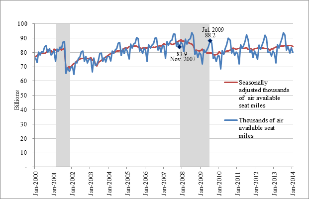
NOTES:Available seat miles from all U.S. air carrier domestic and international, scheduled passenger flights
Shaded areas indicate U.Southward. recessions, every bit defined past the National Bureau of Economical Enquiry. Run into: http://world wide web.nber.org/cycles.html(link is external)
SOURCE:U.S. Section of Transportation, Agency of Transportation Statistics, https://world wide web.transtats.bts.gov/OSEA/TSI/
Unadjusted versus Seasonally-adjusted Data: An Example
Applying seasonal aligning to BTS airline information illustrates its usefulness. The following more than detailed example shows how seasonal adjustment tin be used to wait at existent changes in RPMs. The adjusted and unadjusted information used in the post-obit example tin be institute hither.
Seasonally-adjusted data help uncover brusque and long-term trends in RPMs. Short and long-term trends in the airline industry traditionally have been depicted by year-over-year changes in unadjusted data. These comparisons brim around the influence of seasonal movements by comparing the same month (e.g., May to May) only are flawed for two reasons. Commencement, the months may be disparate because of calendar effects, e.grand., one may contain Easter while the other does not. 2nd, variation may occur betwixt the months; at that place may be an overall rising (decline) between the months simply some refuse (growth) within. For instance, RPMs rose between May 2012 and May 2013 but did not climb steadily. This is difficult to encounter when looking at unadjusted numbers because of seasonal movement (due east.thousand., RPMs ascent naturally in the summer as holiday-related travel rises). When seasonally-adjusted, information technology tin can be seen that RPMs rose but not steadily from May 2012 and declined between February and March, only rise one time once more in May just above the February 2012 number (run across table 3).
TABLE 3. Revenue PASSENGER MILES (RPMS), MAY 2012-MAY 2013
(Thousands)
| Date | Unadjusted | Seasonally-adjusted | ||
|---|---|---|---|---|
| Value | Per centum alter | Value | Percentage change | |
| May-2012 | 71,155,609 | 68,360,655 | ||
| June-2012 | 76,014,162 | 6.8 | 68,491,139 | 0.2 |
| July-2012 | 79,640,786 | iv.eight | 68,140,804 | -0.v |
| August-2012 | 77,738,861 | -2.4 | 68,705,504 | 0.8 |
| September-2012 | 65,230,938 | -xvi.one | 68,477,562 | -0.3 |
| Oct-2012 | 66,974,008 | 2.vii | 68,311,549 | -0.two |
| November-2012 | 63,372,211 | -5.four | 68,800,874 | 0.7 |
| December-2012 | 65,923,928 | 4 | 68,809,269 | 0 |
| January-2013 | 62,433,152 | -5.iii | 69,357,012 | 0.8 |
| Feb-2013 | 57,526,035 | -seven.ix | 70,010,282 | 0.9 |
| March-2013 | 72,164,049 | 25.four | 69,375,821 | -0.9 |
| April-2013 | 67,827,663 | -6 | 69,587,244 | 0.3 |
| May-2013 | 72,980,842 | seven.vi | lxx,067,688 | 0.vii |
| Year-over-twelvemonth change | ii.6 | 2.5 | ||
NOTES: Acquirement passenger miles from all U.South. air carrier domestic and international, scheduled rider flights
SOURCE: U.South. Section of Transportation, Agency of Transportation Statistics, https://www.transtats.bts.gov/OSEA/TSI/ as of May ix, 2014
Seasonal adjustment controls for calendar effects and information outliers and removes seasonal effects. The model developed by BTS to seasonally arrange RPMs detects and controls for agenda effects and outliers nowadays in the information before seasonally adjusting the data. Looking at year-over-twelvemonth changes in the unadjusted and adjusted data bear witness how inaccurate pictures may be drawn from the unadjusted data; there are significant differences in the estimated changes. This can be seen conspicuously in making year-over-year comparisons for the month of March, as an case. RPMs tend to increase in March when Easter occurs in that month. Easter, even so, may occur in March in one year and April in the following year. Thus, year-over-year comparisons of revenue passenger miles for March are misleading when the upshot of Easter is not taken into account. Easter is a holiday that was plant by BTS to significantly influence RPMs and is controlled for in the model used to seasonally adjust RPMs.
Tabular array four shows the yr-over-year alter in RPMs for the unadjusted and adapted serial for the month of March from 2000 to 2013. Year-over-yr changes in unadjusted RPMs are noticeably different from the adjusted values when a March without an Easter occurrence is compared to one with (these values are bolded in Table 1). The divergence is virtually noticeable in comparing March 2004 with March 2005. The unadjusted data suggests RPMs increased xi.0 percent from March 2004 to March 2005. This increment is due, partially, to the occurrence of Easter in March 2005 which spurred holiday-related travel and thereby boosted RPMs above the March 2004 level, which was unaffected by Easter related travel. If Easter is taken into account, as in the seasonally-adjusted information, the increase is only viii.7 pct: 2.3 percentage points lower than the value calculated from the unadjusted data.
Table iv. UNADJUSTED AND SEASONALLY-ADJUSTED REVENUE PASSENGER MILES FOR THE Month OF MARCH, 2000-2013
| Brainstorm date of Easter travel | Easter date(1) | End date of Easter travel | Thousands | Year-over-twelvemonth percent change | Percent-age point deviation | |||
|---|---|---|---|---|---|---|---|---|
| Unadjusted | Seasonally- Adjusted | Unadjusted | Seasonally- Adjusted | |||||
| 2000 | NA | NA | NA | 59,632,015 | 56,801,077 | |||
| 2001 | NA | NA | NA | 60,769,074 | 58,100,149 | 1.9 | 2.3 | 0.4 |
| 2002 | iii/28/2002 | three/31/2002 | 4/two/2002 | 56,037,382 | 52,708,478 | -7.8 | -9.iii | one.5 |
| 2003 | NA | NA | NA | 54,994,261 | 52,763,526 | -1.9 | 0.one | -1.viii |
| 2004 | NA | NA | NA | 61,923,381 | 59,610,118 | 12.six | 13.0 | 0.iv |
| 2005 | 3/24/2005 | iii/27/2005 | 3/29/2005 | 68,725,711 | 64,789,311 | 11.0 | 8.7 | -two.3 |
| 2006 | NA | NA | NA | 69,483,899 | 66,708,174 | 1.1 | 3.0 | 1.nine |
| 2007 | NA | NA | NA | 71,497,177 | 68,851,912 | 2.9 | iii.2 | 0.three |
| 2008 | 3/20/2008 | 3/23/2008 | 3/25/2008 | 73,427,185 | 69,746,721 | ii.vii | i.iii | -1.iv |
| 2009 | NA | NA | NA | 65,147,741 | 63,222,826 | -11.3 | -9.iv | -1.9 |
| 2010 | NA | NA | NA | 67,304,853 | 65,469,595 | iii.iii | 3.6 | 0.2 |
| 2011 | NA | NA | NA | 69,104,312 | 67,294,729 | 2.vii | 2.8 | 0.1 |
| 2012 | NA | NA | NA | 70,799,480 | 68,884,609 | 2.5 | ii.4 | -0.1 |
| 2013 | three/28/2002 | iii/31/2013 | iv/ii/2013 | 72,164,049 | 69,375,821 | i.ix | 0.7 | -1.two |
(ane) NA where Easter holiday does not occur in the month of March
NOTES:Revenue passenger miles from all U.S. air carrier domestic and international, scheduled passenger flights
SOURCE: U.S. Department of Transportation, Agency of Transportation Statistics, https://www.transtats.bts.gov/OSEA/TSI/ as of May 9, 2014
Vacation effects are not necessarily isolated to a single month when looking at transportation data. Travel tends to increase earlier and later on the holiday and not merely on the vacation itself. When a holiday occurs towards the first or end of a month, increases in travel may be observed in the month prior or the month after, respectively. This creates an boosted problem in making yr-over-twelvemonth comparisons in the presence of a moving vacation similar Easter. Years where the holiday is present in neither month may be afflicted by these spillover effects – that is data values may be higher because of pre- or post-holiday travel induced by the vacation occurring in the next or previous calendar month, respectively.
In developing the model to seasonally adjust acquirement passenger miles, BTS constitute a significant increase in rider air travel the iii days prior to through the ii days after Easter1. When Easter occurs tardily in March, as in 2002 and 2013, travel induced past the Easter vacation spills over into April (come across Table 4). Without aligning, there is a i.ix per centum rise in RPMs from March 2012 to March 2013. Using seasonal adjustment to account for the holiday, the increase drops to 0.7 percentage.
There is no spill-over upshot in the years from 2000 to 2013 from Easter occurring in Apr because the entire Easter holiday travel menstruation took place in the calendar month of April without spilling over into March or May. Unadjusted data for the month of April, however, cannot exist accurately compared beyond years considering not all Aprils contain Easter and considering some (April 2002 and 2013) are affected by Easter-related travel spilling over from March into Apr.
Year-over-year comparisons are fabricated more accurate when using seasonally-adjusted data considering seasonal adjustment controls for calendar furnishings and data outliers. Considering seasonal adjustment removes seasonal furnishings, data can be compared across months and years straight. This comparing tin can be misleading with unadjusted data. Seasonal movements in unadjusted data make it difficult even to run into trends within the data. Effigy 1, which shows unadjusted and seasonally-adapted acquirement passenger miles, demonstrates this. Seasonal movement causes RPMs to vary significantly inside a twelvemonth. RPMs tend to climb in the summer months because of vacation related travel; they then fall through the winter months, reaching a low in Feb. This seasonal movement makes information technology difficult to see RPMs are growing or declining. Yet, one time the seasonal-aligning process accounts for seasonal motion, information trends can be seen more than readily – equally in Effigy 1 for RPMs – and computed across all months and years. The adjustment gives a more nuanced picture of the data than year-over-year comparisons.
Effigy 2. REVENUE Rider MILES, January 2000 TO January 2014
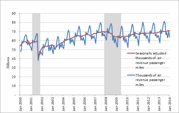
NOTES:Acquirement rider miles from all U.S. air carrier domestic and international, scheduled passenger flights
Shaded areas signal U.S. recessions, as defined past the National Bureau of Economical Inquiry. See: http://www.nber.org/cycles.html(link is external)
SOURCE:U.S. Department of Transportation, Bureau of Transportation Statistics, https://www.transtats.bts.gov/OSEA/TSI/ as of May 9, 2014
Summary
Seasonally-adjusted data help uncover real monthly changes; short and long term patterns of growth or decline; and turning points. Unadjusted data tin can be misleading when used to measure these types of underlying changes because of calendar related furnishings.
1 The Bureau of Transportation Statistics referred to industry experts in determining the number of days earlier and after a holiday when vacation traffic is expected. This was used to create a parameter in the seasonal adjustment model. Various parameters were tried until finding the about significant parameter and best fitting model.
Source: https://www.bts.gov/explore-topics-and-geography/topics/seasonally-adjusted-data-what-it-really-means
0 Response to "What Does It Mean to Seasonally Adjust Data"
Postar um comentário